
The CellView Lens includes a machine learning platform that allows you to train a convolution neural network (CNN) to divide a selected population into two classes using only patterns identified in the images.
Installing Machine Learning Tools
When you install and run the CellView Lens plugin, the doML and doTiffExtraction packages will unpack into the CellViewExt folder, in an operating system dependent subfolder called either OSX (Mac) or Win (Windows):
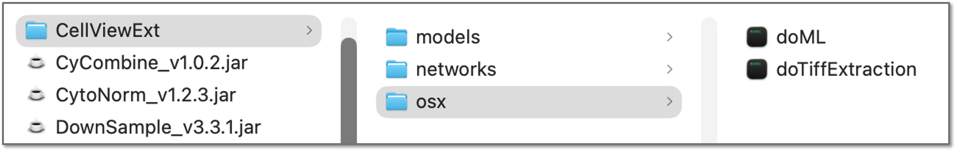
Figure 1: Folder structure of ML tools, shown on a Mac
If the additional tools fail to automatically unpack they can be downloaded directly and arranged to match the folder structure above. Additionally, the networks folder will be created and it will include three CNN models that will be your starter set of networks to choose from:
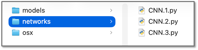
Figure 2: CNNs in the networks folder
These CNNs are written in plain text in the Python programming language. Advanced users can open any of them in a text editor and modify the structure of the CNN in a fairly straight-forward manner by changing the number of layers, neurons, or the activation function of a layer to create new neural net variants.
The Machine Learning (ML) Dashboard
To access the ML dashboard, open a CellView Lens node on any population. The ML dashboard is the gear-head icon in the bottom righthand corner of the CellView window:

Figure 3: ML Icon
Clicking the icon reveals a dashboard with three tabs that can be used in sequence: Train New Model, Classify Subpopulations, and Show Results.
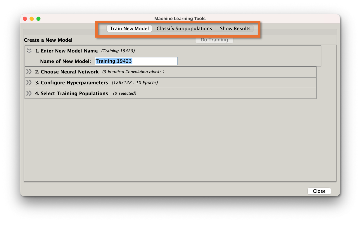
Figure 4: ML Dashboard
Train New Model
Training a new model is a five step process, with the steps corresponding to the numbers in Figure 5:
- Give you model a name. In this example I'm attempting to identify B and T cells interacting from a population of doublets, some of which are cells interacting, some of which are just two separate particles caught in the same droplet, some of which are other cell types interacting.
- Choose a neural network. The three default networks are shown here. Each are reasonable choices but we have not done extensive testing to recommend the conditions under which to use one versus the other. The information displayed about each network is:
- Layers - the number of layers with the number of neurons per layer
- Loss Function - the metric used to evaluate network performance
- Last Activation - the activation function used in the output layer.
- Configure Hyperparameters. Hyperparameters are the settings used to train the network.
- The number of Epochs determines how many cycles of adjusting the weights within the network will be used. Adjusting the number upward will cause the network to do a better job on the training data at the risk of overfitting the network to specifically the training data. Lowering it will make a less accurate but perhaps more generalized network. The consistency of the data you will use the network to classify is the deciding factor.
- The maximum number of images per population is a limiting factor to cap the size of the input data.
- The data width settings allow you to present the networks images of uniform sizes, so that the size of the image is not the determining factor in classification. To make the images a uniform size, smaller images need to be padded. If you have lightloss turned on the background will be a mix of gray scale pixels, making 'Pad with Random' a good option. If you have lightloss turned off and have a uniform black background, 'Pad with black' is the best choice. If you have inverted the image then 'Pad with white' is the best choice.
- Concatenate channels horizontally combines all enabled channels into one single image, with separate channels placed side-by-side.
- Interleave channels vertically makes a single image by separating the channels and weaving each row of each channel into a sequence vertically.
- If neither of those options are chosen, the images will be used holistically.
- Select training populations. The network needs to be shown an example of each type of cells you want to find. The best way to do this is to use image sets to manually curate a set of images that all look like the target population. You will need at least two target populations to allow the network to learn differentiating features. In the two population case, we recommend deliberately picking out a set of images that do not look like your target rather than simply accepting the NOT gate automatically created by image sets. NOTE: CellView Lens will display all populations that have a CellView Lens node applied to them. Nodes can simply be dragged to each population you would like to use in the FlowJo hierarchy.
- Start the training.
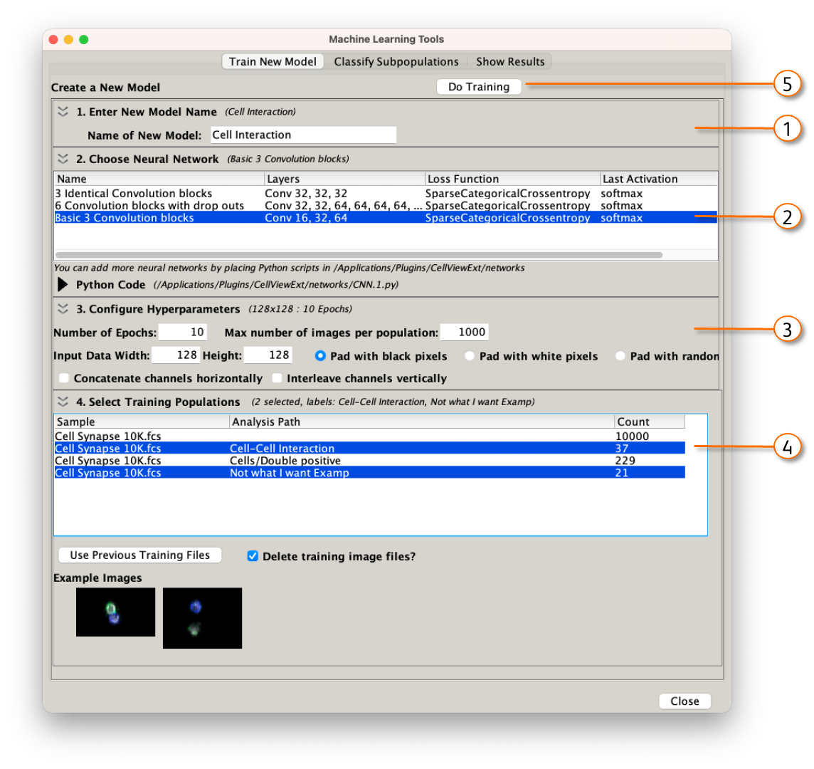
Figure 5:Train a model
Classify Subpopulations
When you train a network, a model gets written into the {Workspace name}/BD CellView Lens/models folder. These are accessible within the workspace to be applied to any population and can be ported to other workspaces either by dragging the model folder into the folder of another workspace or using the Add Model button in the Classify tab. NOTE: To run a network on other data, the same parameters should be present.
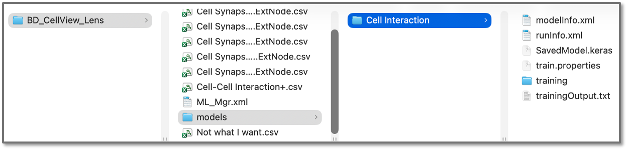
Figure 6: Saved model
To classify a population with a trained model, go to the Classify Subpopulations tab within the ML dashboard. There are four steps to classifying, with the steps corresponding to the numbers in Figure 7:
- Select the population that you would like to run the classification on.
- Select the model that you would like to use. CNN, training accuracy and loss, and validation accuracy and loss are displayed for each model, and are available as graphs if the 'Show...' widget is expanded. Higher accuracy is better, and lower loss is better.
- Enter a probability threshold for classification. Most output layer activation functions assign a probability of being in the desired class to each cell. You can adjust that probability here with the default being 90%.
- Run the model.
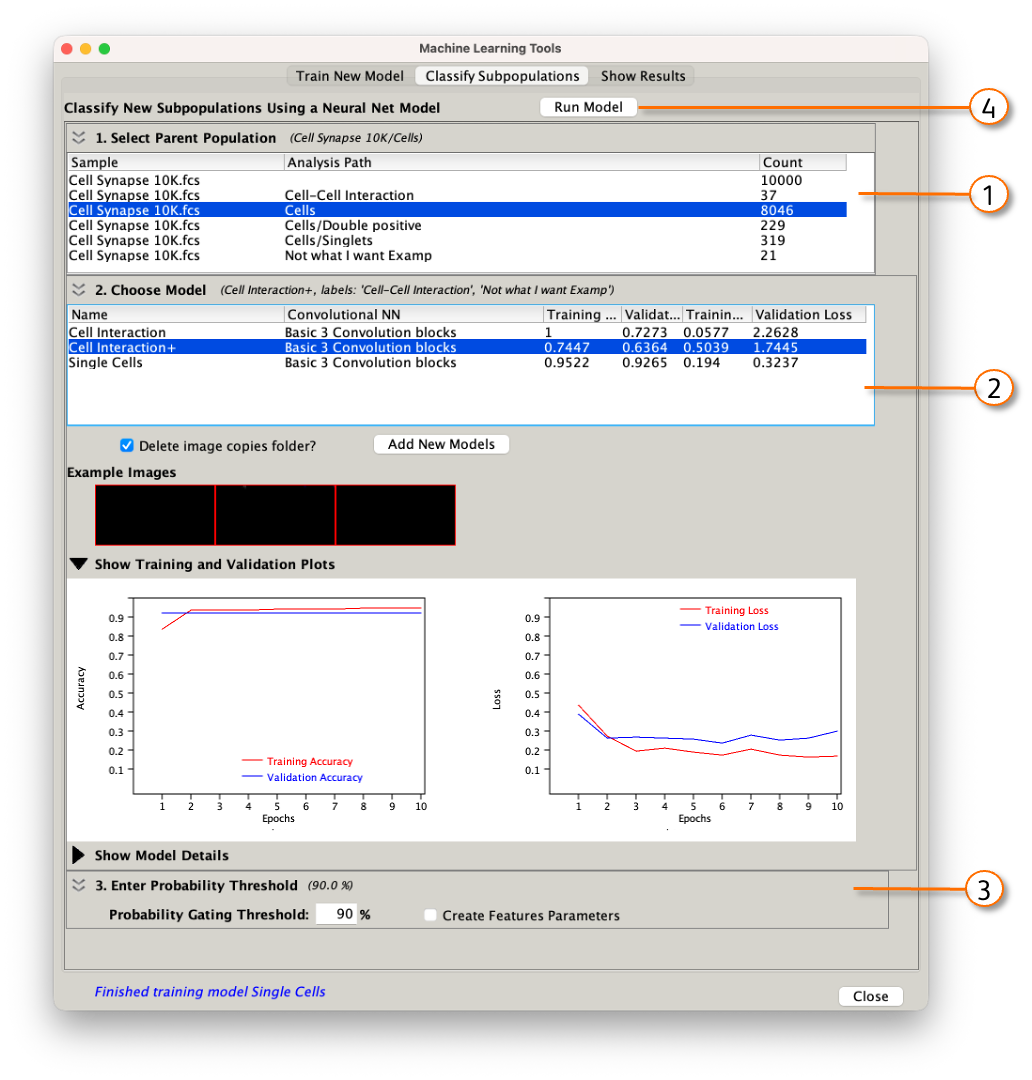
Figure 7: Classifying a population
Show Results
The show results tab will allow you to pick a classification and show the probabilities of each cell belonging to a particular class, and the gates identifying those cells.
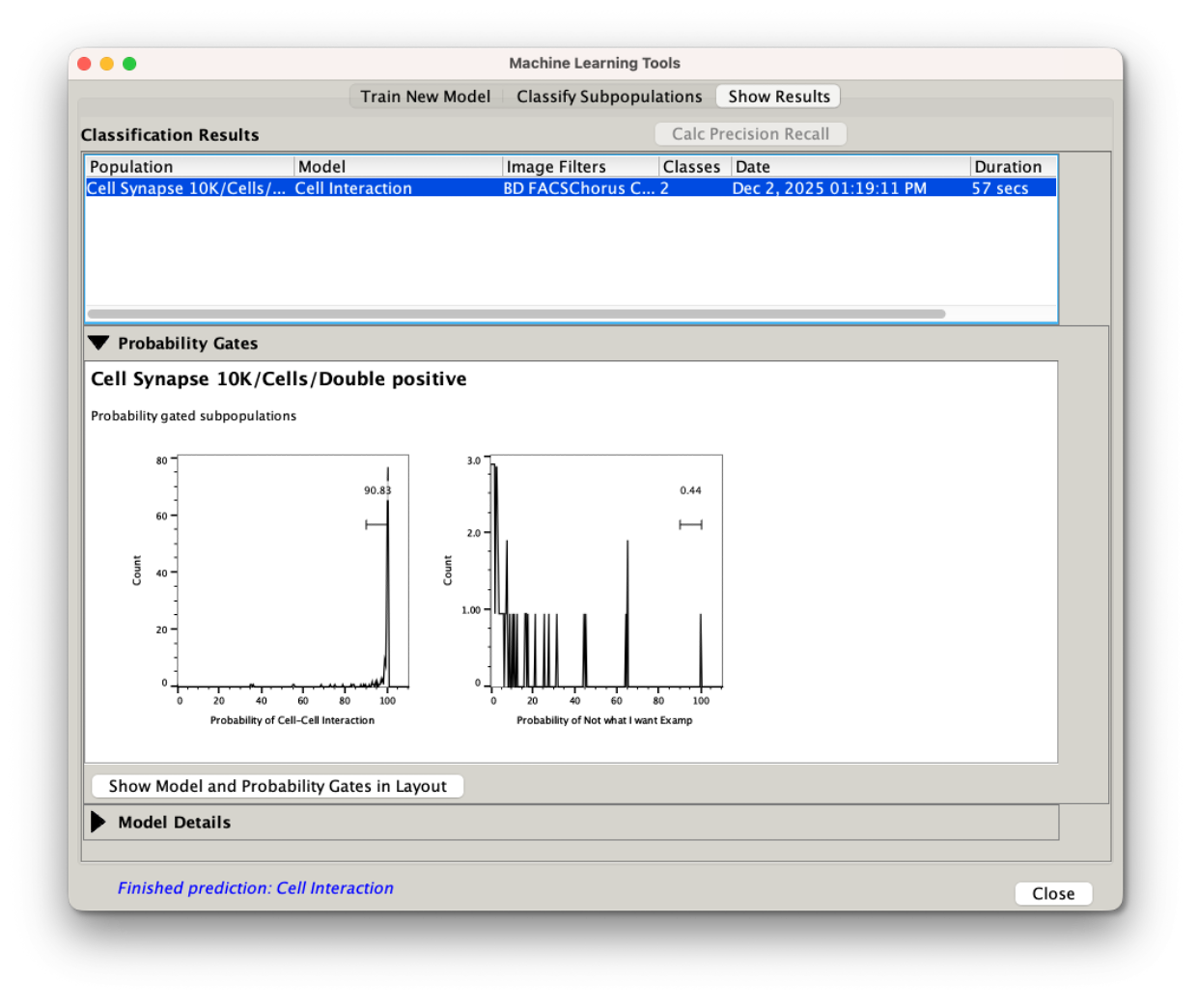
Figure 8: Displaying results
Additionally, the classification process produces two sub-populations from the population selected for classification, one matching each example population. They will be named 'Probability' {model name} {population to be classified} {example population name}. This name is information rich but lengthy, and you may use the rename function (Ctrl or Cmd + R) to create more succinct names. In this example we have used a CNN to hunt through our population of cells positive for both B and T cell markers and find the pairs that were near each other and found that 90% of this small population were touching.
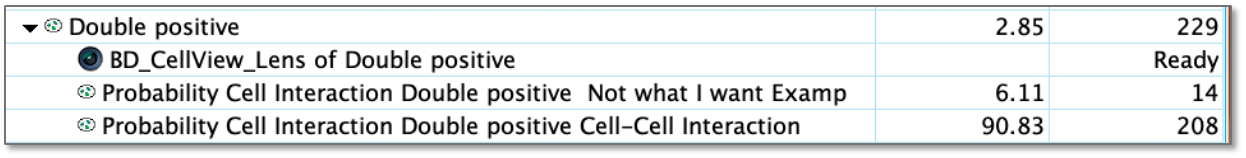
Figure 9: Populations created in the FlowJo hierarchy